CFD Workflow
I want to get more into the specific CFD workflow the team and I followed this season. The following serves as a blend of business-casual documentation, and a tutorial for future members of the team.
Geometry Cleanup in Ansys SpaceClaim
Taking the simplified CAD model from Suspension Considerations for Aerodynamics we export a STEP AP214 file and import it into Ansys Fluent. From here, we use various tools to clean up the geometry and preapre it for meshing.
I prefer to use Fluid Flow (Fluent with Fluent Meshing) since it has a very nice integrated workflow for both pre and post-processing.
First order of business is to use SpaceClaim. I haven’t had good experiences with the stability of Discovery, and DesignModeler is very old at this point. SpaceClaim is relatively more stable from my experience, and after using it 30-40 times over it becomes intuitive.
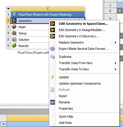
Fig. 1 Use SpaceClaim, it causes the least headaches (as long as you know how to use it)
SpaceClaim has a number of great tools to repair geometry. I personally like to run split edgews and extra edges, which usually allows Ansys to find things it doesn’t like. Be sure to use these before performing any meshing to ensure you have an easy time meshing everything.
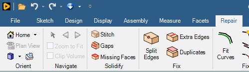
Fig. 2 My preferred SpaceClaim repair tools. You may need to return to this stage and run more tools if you have trouble with meshing down the line
After running repairs I model tire contact patches. Right now these are crude rectangles drawn 2mm underneath each wheel, and extruded upwards. We only need to sketch 2 rectangles on the right-side wheels since we apply the symmetry condition when solving.
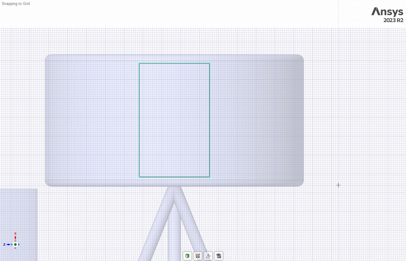
Figs. 3 and 4 Sketching and pulling crude rectangles to model tire contact patches. This stage of the process needs optimizing (i.e. is there a better way to do this?)
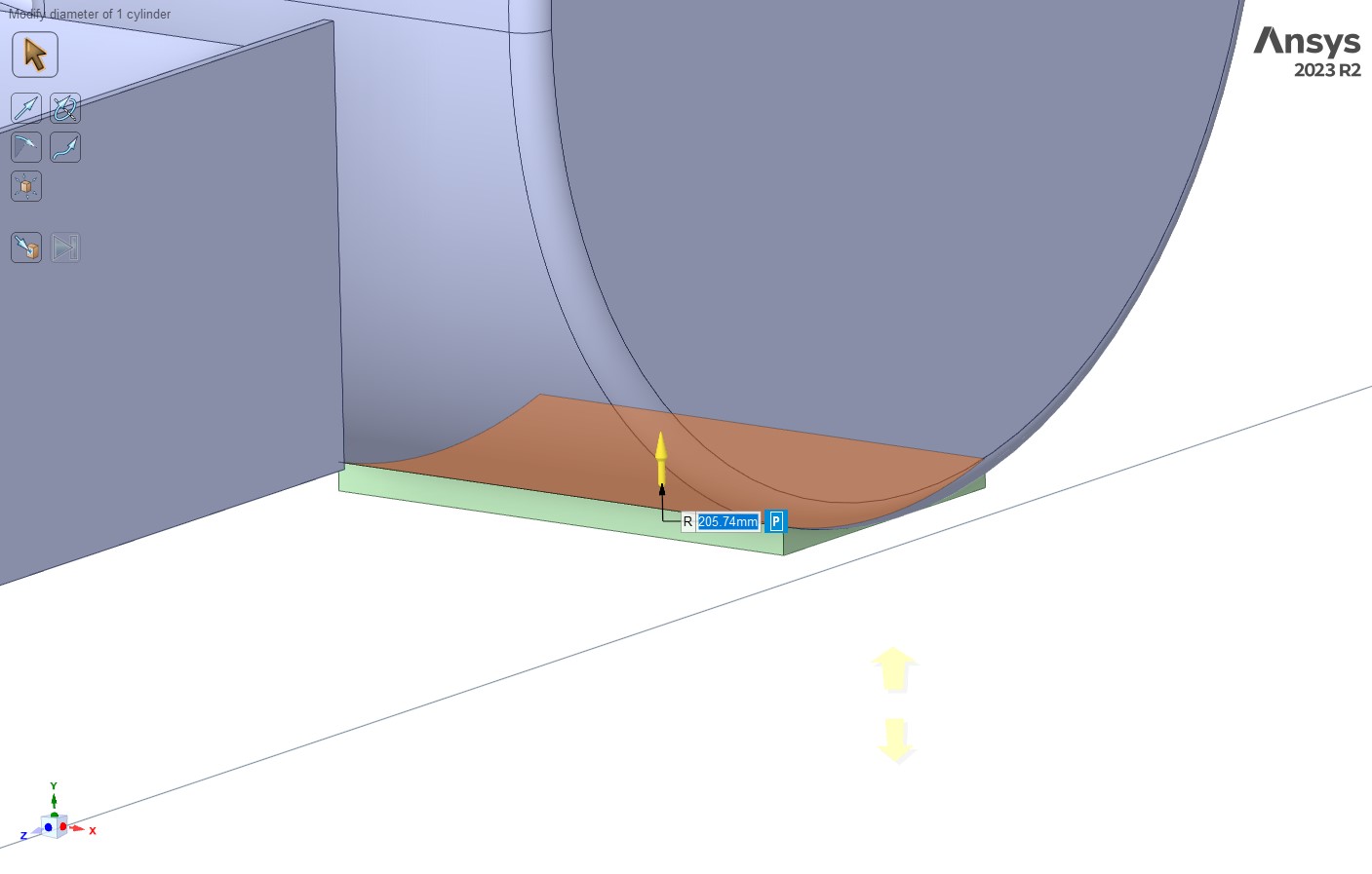
Next create a symmetry plane, easy enough to do. After that, model an enclosure using the enclosure tool. Decent dimensions are given below however “decent” is not an engineering term. We need to research blockage ratios for next season and understand how to properly model a virtual tunnel to avoid artificial acceleration of the fluid.
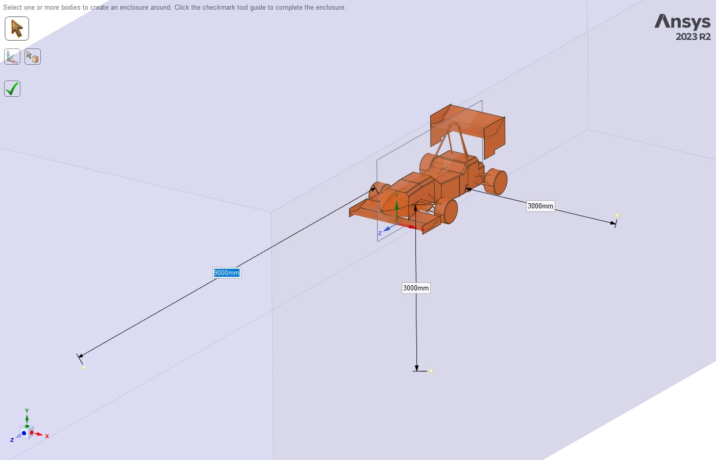
Fig. 5 EV5 tunnel sizing. Needs to be researched and improved
Ansys should have processed the enclosure nicely if you repaired your geometry well enough. If it didn’t work, undo your enclosure and go back to the repair tab and use more repair tools. If that doesn’t work, go back to SW since something is most likely fundamentally messy about your model.
Hide the enclosure and ground plane and make a rectangular sketch on the symmetry plane which roughly encompasses the model. No dimensions needed for this part. Pull the rectangle out to create your boi-nearfield which will be used for mesh refinement. Create a copy of your nearfield, pull out the whole cube by an additional 500mm and name it boi-farfield. You should have 2 rectangular prisms now, the nearfield and the farfield.
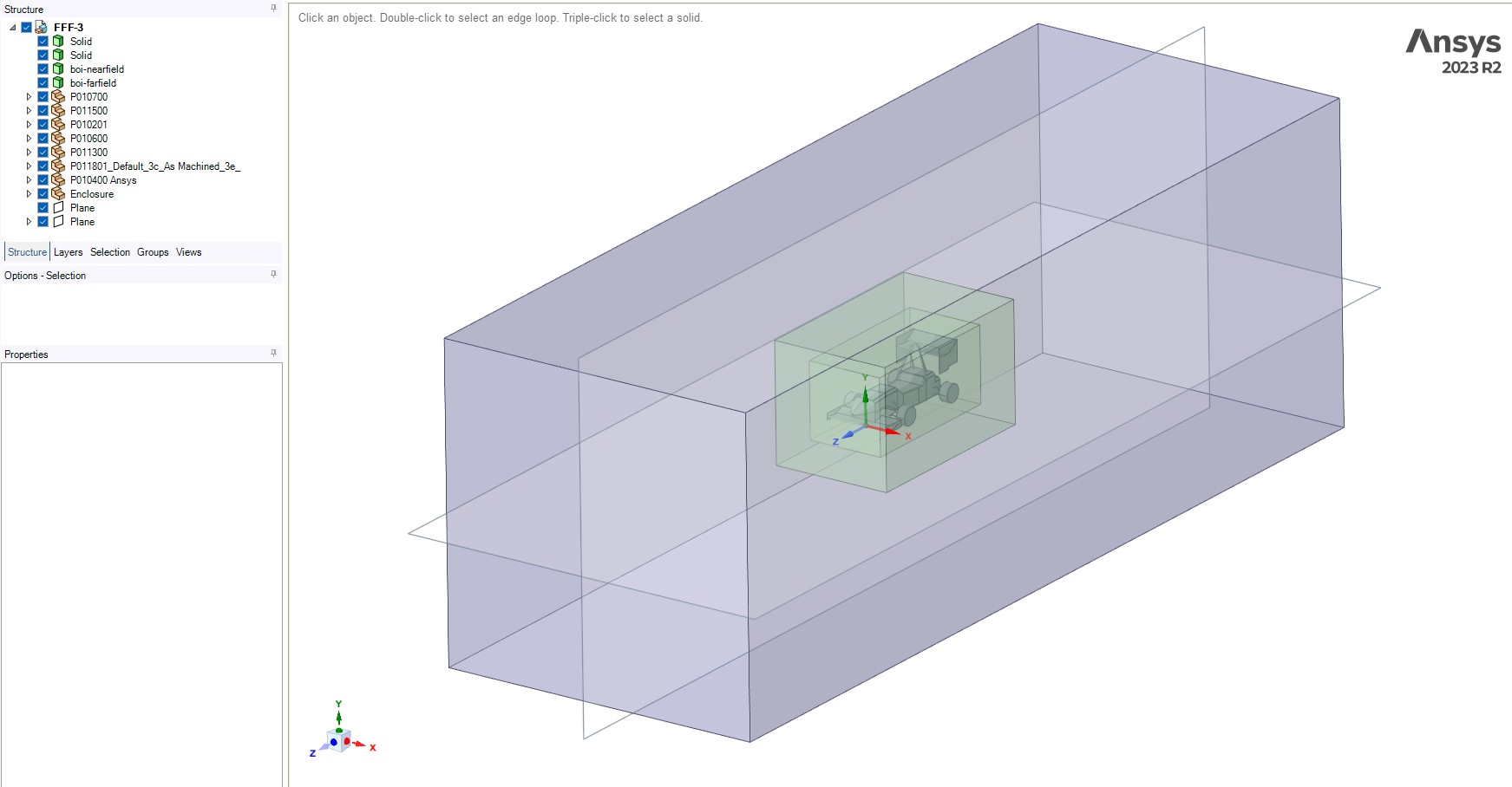
Fig. 6 Everything we have so far. Make your BOIs transparent to check if everything looks good inside of them
Now comes some optimization. We cut the tunnel at the symmetry and ground planes to reduce compute and model ground effect, respectively. Use the split body tool for this.
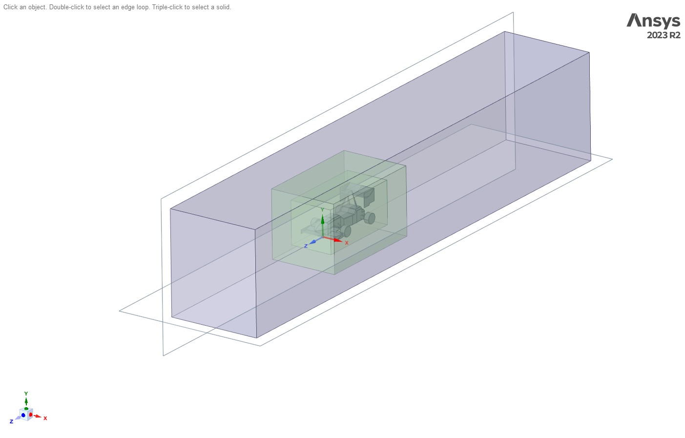
Fig. 7 Final tunnel
Hide the planes, CAD, the 2 solid bodies for the contact patches we modelled, and suppress both the CAD and contact patches for physics since the enclosure has already captured a negative of the entire model.
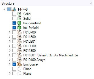
Fig. 8 Right click to suppress physics
Go to groups and start making your named selections. Below are mine which I recommend following, since I’ve broken it down to make meshing easier later on. Double check the surfaces you are highlighting, as it is very easy to add the same surface to 2 unique NS, or to completely miss out on a surface altogether. This step requires practice and extreme patience. Get this right.
Fig. 9 Named selections
Ctrl-S, close SpaceClaim and you’re good to start meshing.
Meshing and Mesh Sensitivity
Import your geometry and add local sizing. This is the stage where we’re going to make a refined mesh for each part of the car.
After having to spend 2 weeks learning how to setup a host server for our new Ansys sponsorship, and writing a new installation tutorial for the team (since they didn’t give us one), I wasn’t left with much time to document the mesh sensitivity studies I performed. For now, just take my word on it that for our current models a boi-nearfield of 16mm and farfield of 32mm achieves grid independence to within 5% error of 8mm and 16mm.
As for the surface mesh I found that I could just apply a curvature constraint to every part of the car (i.e. all “car” related named selections from earlier) and this was sufficient in outputting a reasonable answer relative to other FSAE teams running our specific aero configuration. Further refinements can be made and should be explored.
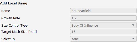
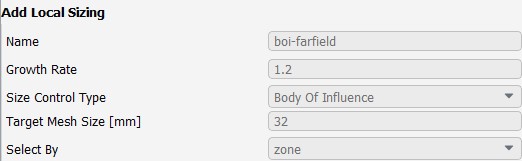
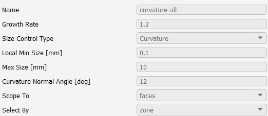
Figs. 10, 11, and 12 Local sizing applied to EV5
Generate a surface mesh of min=0.5mm and max=256mm. One thing to note is I had to change cells per gap to 0.5 since the trailing edges of the airfoils were too thin for Ansys to fit a cell inside. If you chamfer the airfoils by about 2mm instead of 1mm you should be able to fit a full cell. Comparing solutions between these 2 different modelling choices should be studied.
Insert an improve surface mesh task to bring face skewness to 0.7 or below. I tried running a solution at 0.85 and it would’ve taken 5 days to solve. At 0.7 it’s 24 hours for 1000 iterations.
Below is how I described my geometry. Your enclosure should be defined as a fluid.

Figs. 13 and 14 Describing geometry and setting boundary definitions
For boundary layer meshing we’ve been using the last ratio scheme since it was recommended by Ansys. Design freeze was fast approaching and this was something we didn’t have time to research and further justify. Boundary layer modelling needs to be significantly researched for next year for obvious reasons (see: BL separation and wing stall).
Volume mesh min=1mm and max=512mm (increased surface mesh by factor of 2) as per Ansys recommendation. Through experimentation this ensured stability while allowing a solvable solution in an expected amount of time (around 1-2 days) however, like many other things, needs to be understood and explored further.
We improved cell quality to 0.15 after the initial volume mesh and had to call it there. Time to solve.
Solver Setup and Solution
Our solver settings have been pretty standard and we’ve left it that way for our first year of doing aero. Pressure-based, steady solver running k-omega SST with no relaxation for the turbulence model itself, and higher order terms. Second order upwind scheme for momentum and turbulent kinetic energy. Very basic, recommended by Ansys, needs to be understood further.
We’ve been running our inlet velocity at 15m/s since that’s the average FSAE cornering speed. Pressure-based outlet with gauge pressure set to 0. Same turbulent intensities and viscosities for both inlet and outlet.
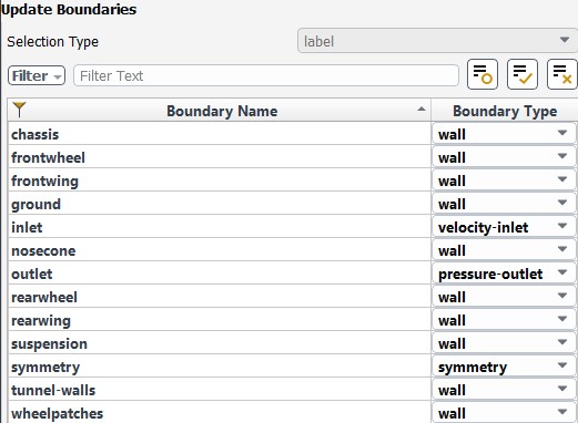
The boundary walls get a little interesting. Translating ground at 15m/s to ensure ground effect plays a part for the front wing/underbody in our solution, and the wheels are rotating as well as can be seen through the setup below. Angular velocity determined through omega=v/r where v=15m/s and r=radius of our tires. Tunnel walls have a zero specific shear to avoid BL growth which could affect flow around the body.
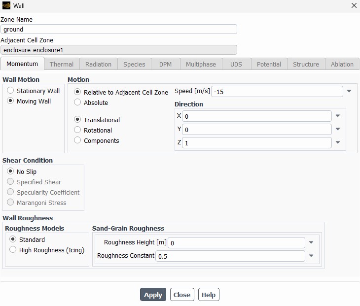

Figs. 15, 16, and 17 Moving boundary walls, namely ground and wheels. Ground is moving in -Z direction since nose faces +Z. Note how the coordinates of the wheels are different for front and rear, this is an important step. Another important thing to note is only the wheel is rotating, not the tire contact patch. This is why they have separate named selections
After this, I set my reference values. A_ref=0.46 since full car is 0.92 (remember we are using symmetry condition). This means the outputted Cl and Cd are that of the full car. Length=3m since this is the length of the car, and v=15m/s. Everything else is untouched.
4 report definitions are setup: Cl, Cd, lift, and drag. I also click the option to create a report file for each so the data can be brought into Excel for analysis.
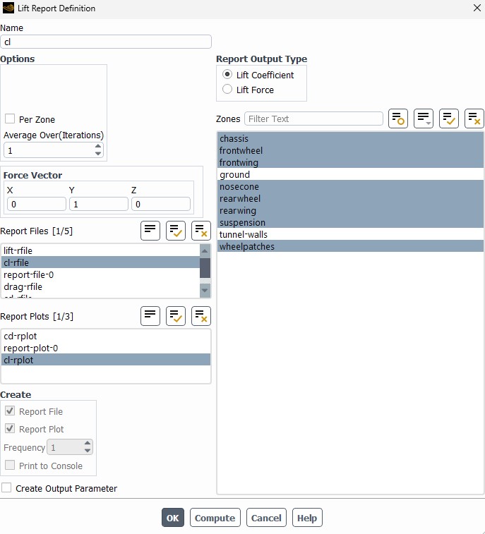
Fig. 18 Cl report definition
I then run the solution for 1000 iterations with an automatic time step. The current assumption is that 1000 iterations is sufficient in providing an accurate enough solution, and this is all we were able to do given the design freeze time constraints this year. In future years, 3000+ iterations should be done to guarantee convergence.
The resulting plots can be seen below.
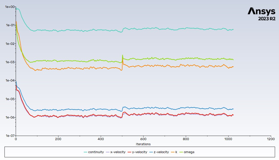
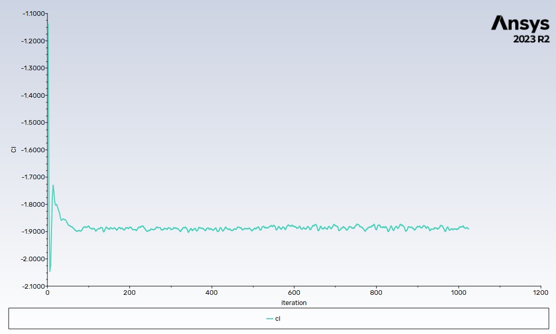
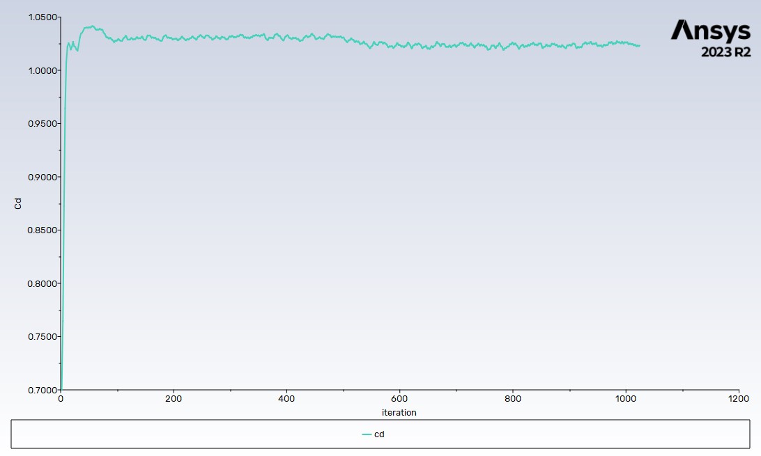
Figs. 19, 20, 21 Resulting plots after 1000 iterations
Post-Processing and Data Analysis
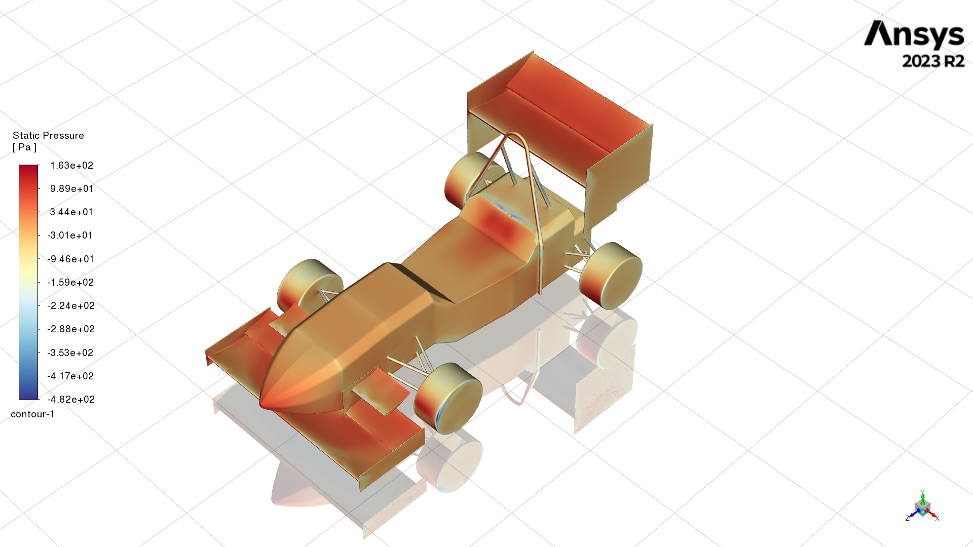
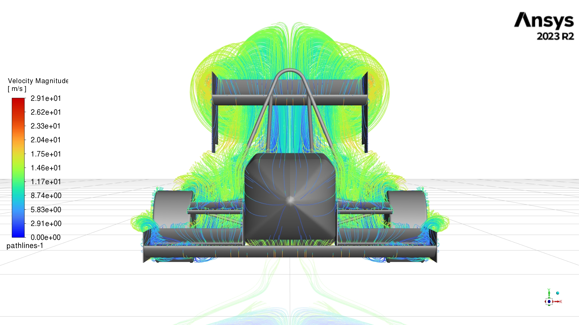
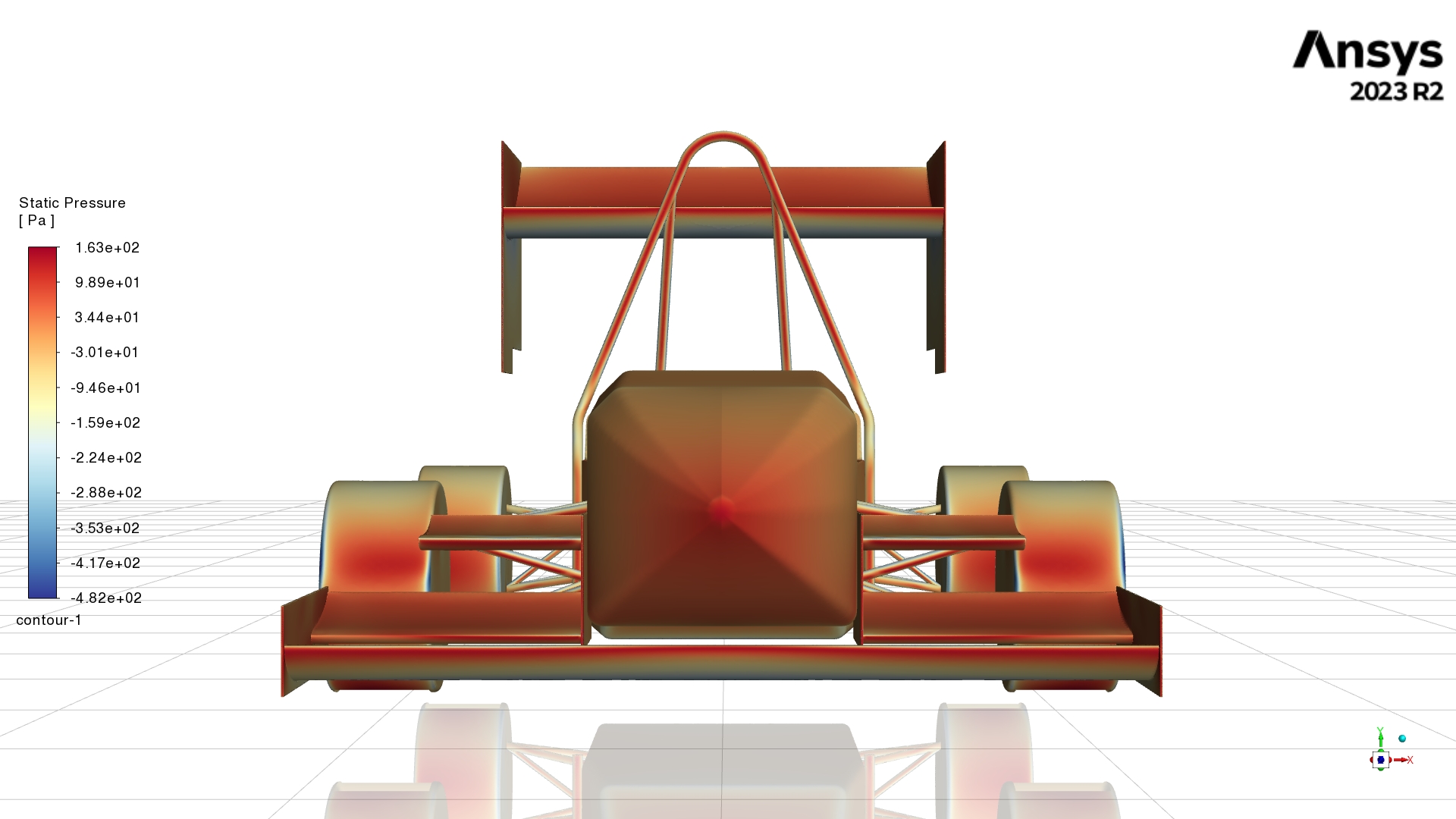
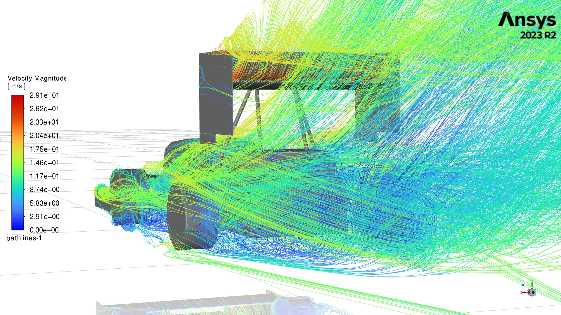
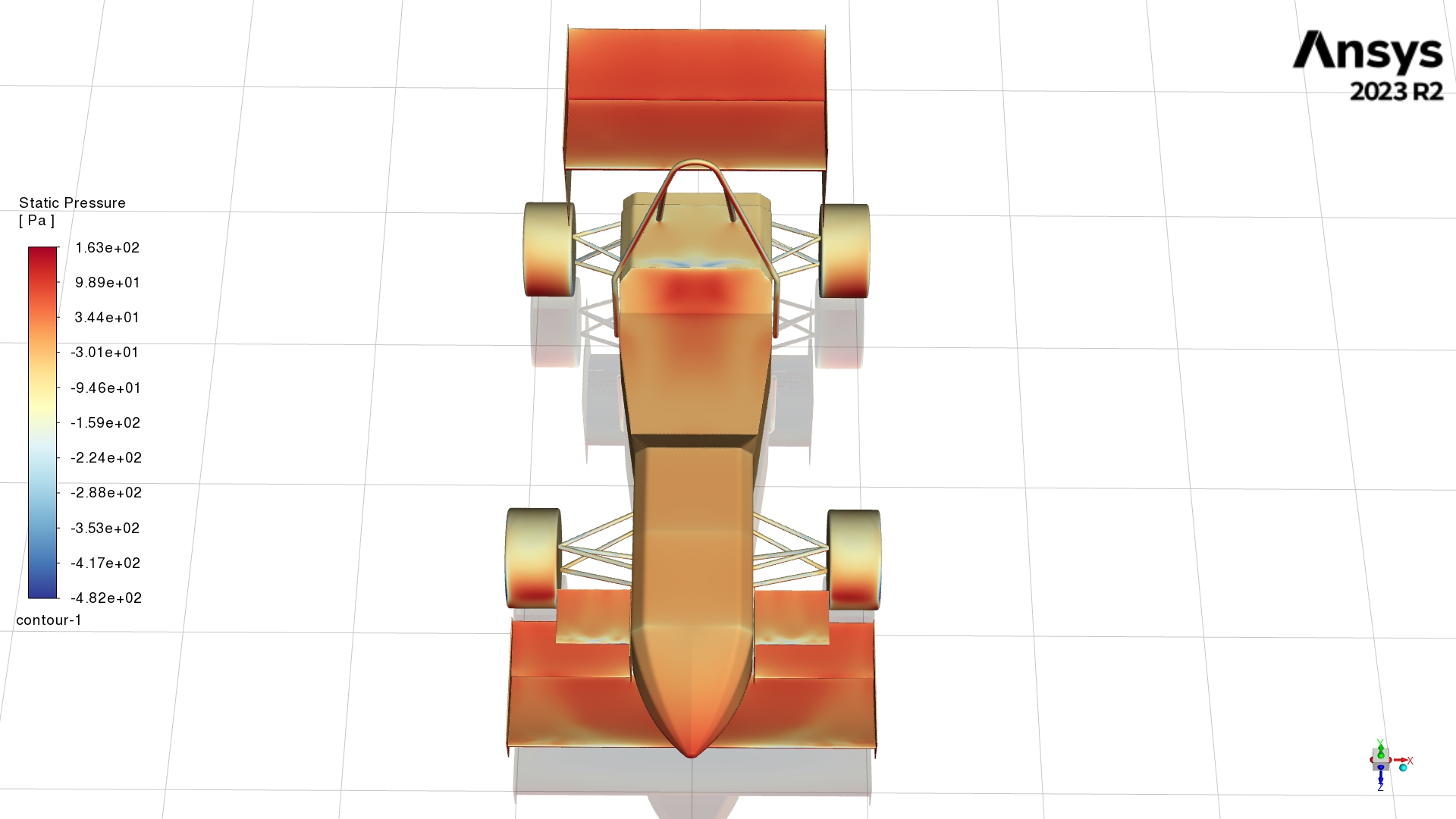
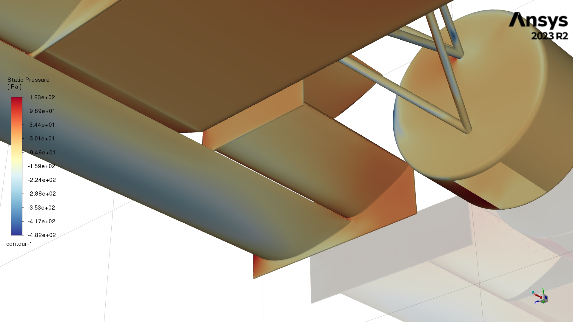
The first order of business is to take some very cool and very useful pictures, because that’s the first thing any hyper-stimulated 20 y/o Adrian Newey wanna-be does at 3:00AM after running a simulation. Also great for marketing!
 |
 |
 |
 |
 |
 |
 |
 |
Figs. 22, 23, 24, 25, 26, 27, 28, and 29 AERODYNAMICS WOOOOOOOOO
Jokes aside, I just don’t know how to extract meaningful results out of velocity pathline images yet. Static pressure plots are more useful to us for design iterations, since we can use them to conceptualize parts that increase/decrease static pressure at various locations. For example, we should look into extending our front wing endplates closer to the ground (suspension allowing) to better seal the outboard portions of the wing, to the benefit of downforce.
The data for Cl, Cd, lift, and drag are outputted to OUT files in this directory.
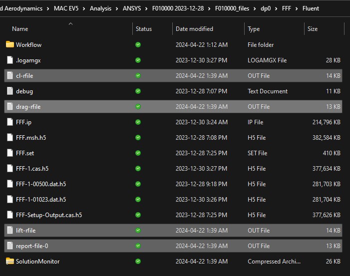
Fig. 30 Outputted files
Import this data into Excel so we can obtain the average. Use the space delimiter with the legacy wizard to get nice data into your workbook. If you don’t use the legacy wizard the data will all appear in one column. Or maybe it’s just a skill issue on my part.
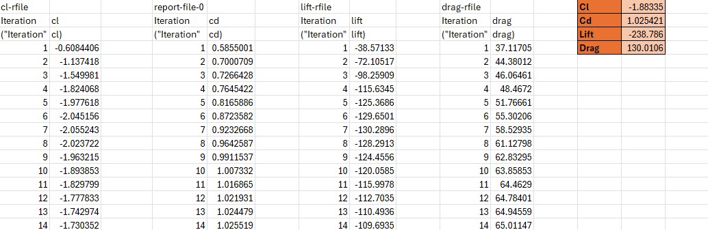
Fig. 31 Importing data into Excel, using AVERAGE function to take average. Multiply lift and drag forces by 2 to get full car forces. Be sure to start taking your average once the forces become more stable, don't take them straight from line 1
This is the extent of our data analysis, and now we’re at the end of the workflow. We primarily use the static pressure images to generate new design concepts, however learning how to use this data to continue to iterate on the design is something we need to learn how to do.
If this post proves anything, it’s that we’ve come a long way, but we still have a long way to go.
It’s 3:35AM, I’m done exams, and the Nordschleife DLC is waiting for me on ACC. Night.