MSES to SOLIDWORKS
2D panel-based methods are far superior to traditional commercial CFD solvers when it comes to numerical accuracy and solution speed. XFOIL and MSES have the added benefit of not having to worry about correct fluid domain sizing and grid refinement. What one student could do in 30 minutes with a commercial solver, the other can do in 3. Mark, I thank you for your genius.
The following serves as an in-depth tutorial for MAC Formula Electric. I hope this makes it clear how to make effective and efficient use of the software.
airset
Go to airfoiltools.com and find your profile(s) of preference. Download the “Selig format dat file” for each profile you will be using. For this tutorial, I will be creating an arbitrary dual-element setup using 2 S1223 profiles.
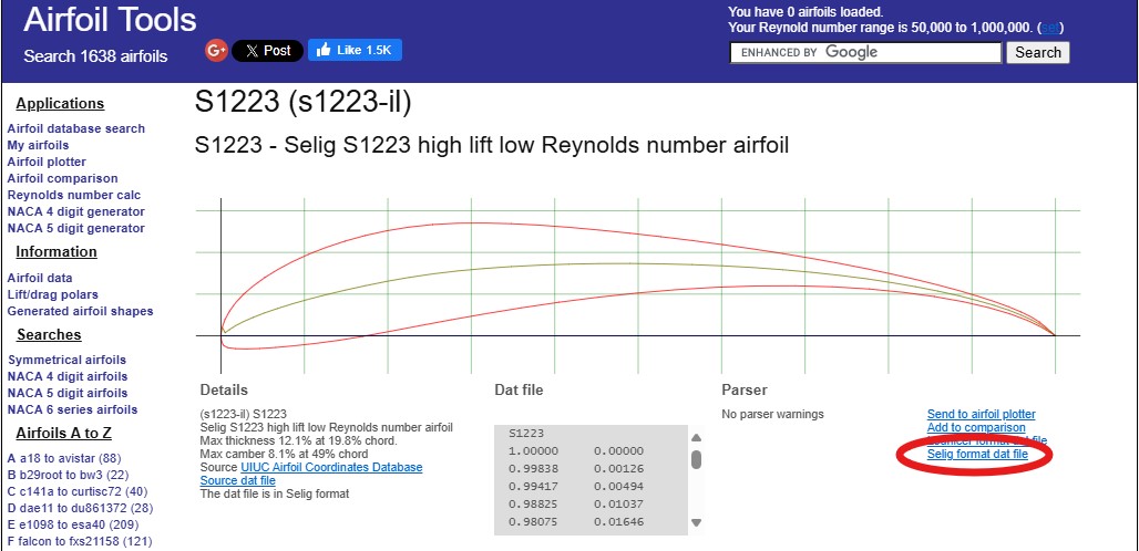
Fig. 1 Selig S1223
Save the file in the same folder as your MSES installation.

Fig. 2 Storing seligdatfile in the directory with all MSES programs
Open airset.
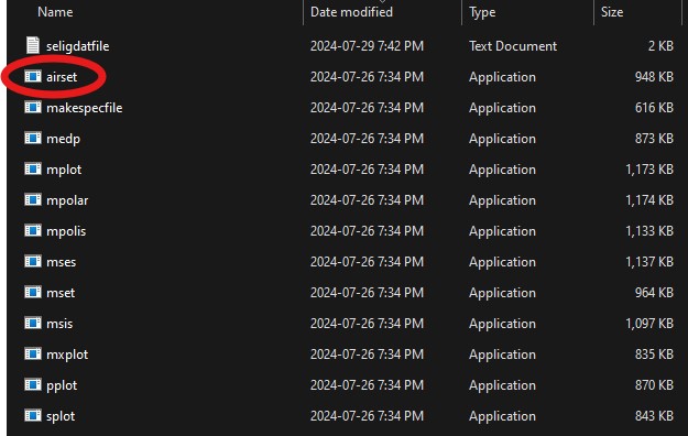
Fig. 3 airset
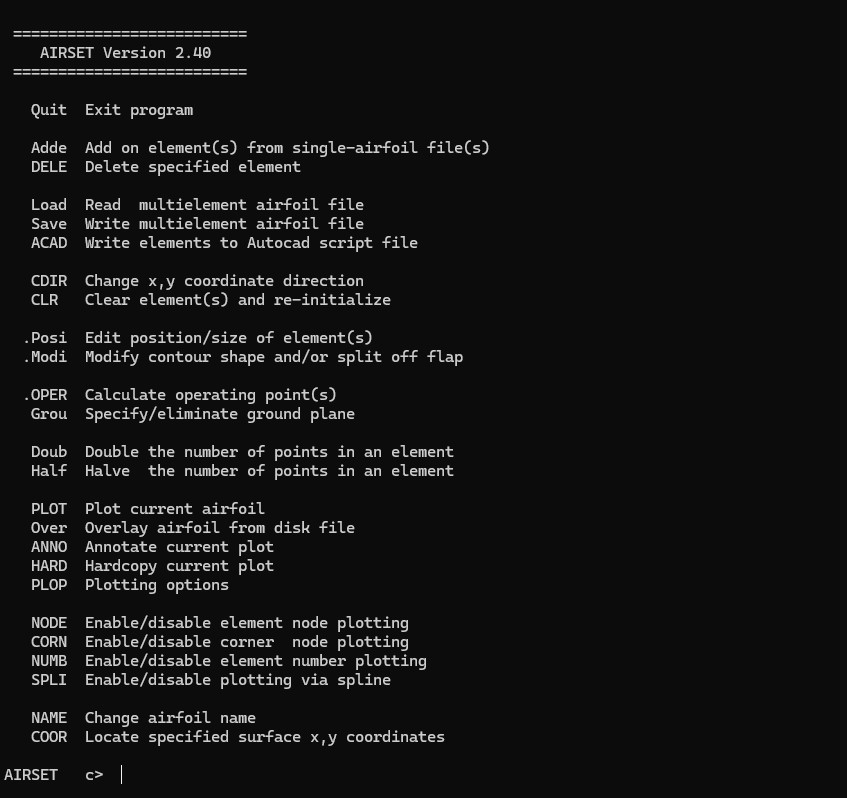
Fig. 4 airset menu
Type “Adde” and hit enter to add the first profile to your setup. Type in the name of the file. You should see a GUI pop up with your airfoil in unit length.
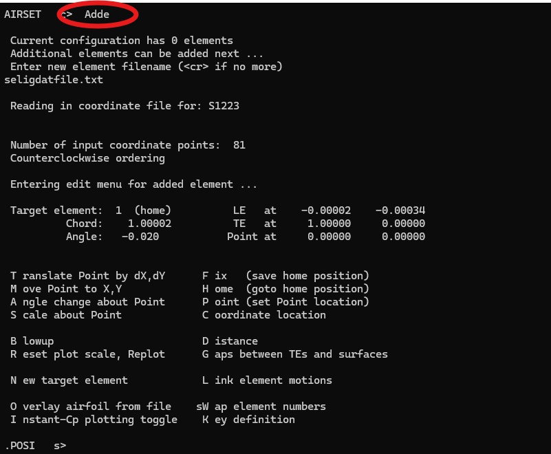
Fig. 5 adde
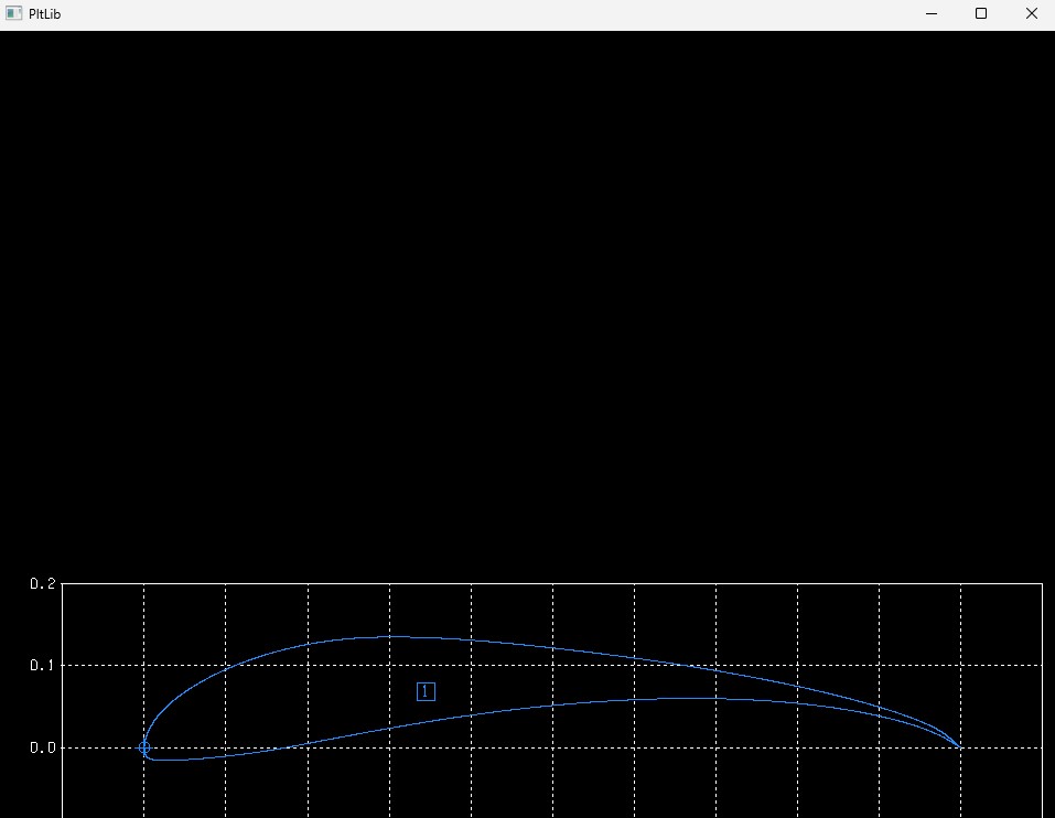
Fig. 6 GUI of airfoil
We are now in the .POSI menu, which can be seen in Figure 3. Type “R” and hit enter to re-size your GUI if it does not sit nicely on your screen.

Fig. 7 Re-sized GUI
There are many commands to enter now, however practically you don’t really want to move the first element away from the origin. Most of the time, you would only want to change the angle of the first element.
So, type “A” and hit enter. Positive values are CW, negative values are CCW. Hit enter.
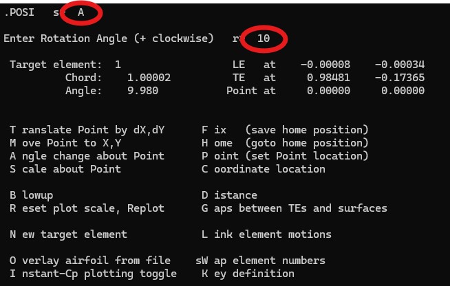
Fig. 8 AoA of +10deg
Once you are happy with your primary element’s AoA, hit enter. You may now enter the filename of the second element. The GUI will now display 2 elements.
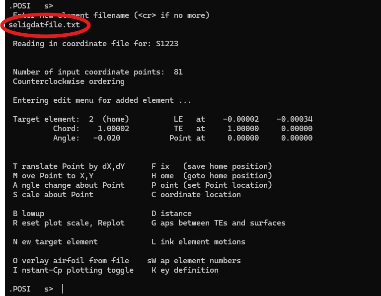
Fig. 9 Second element
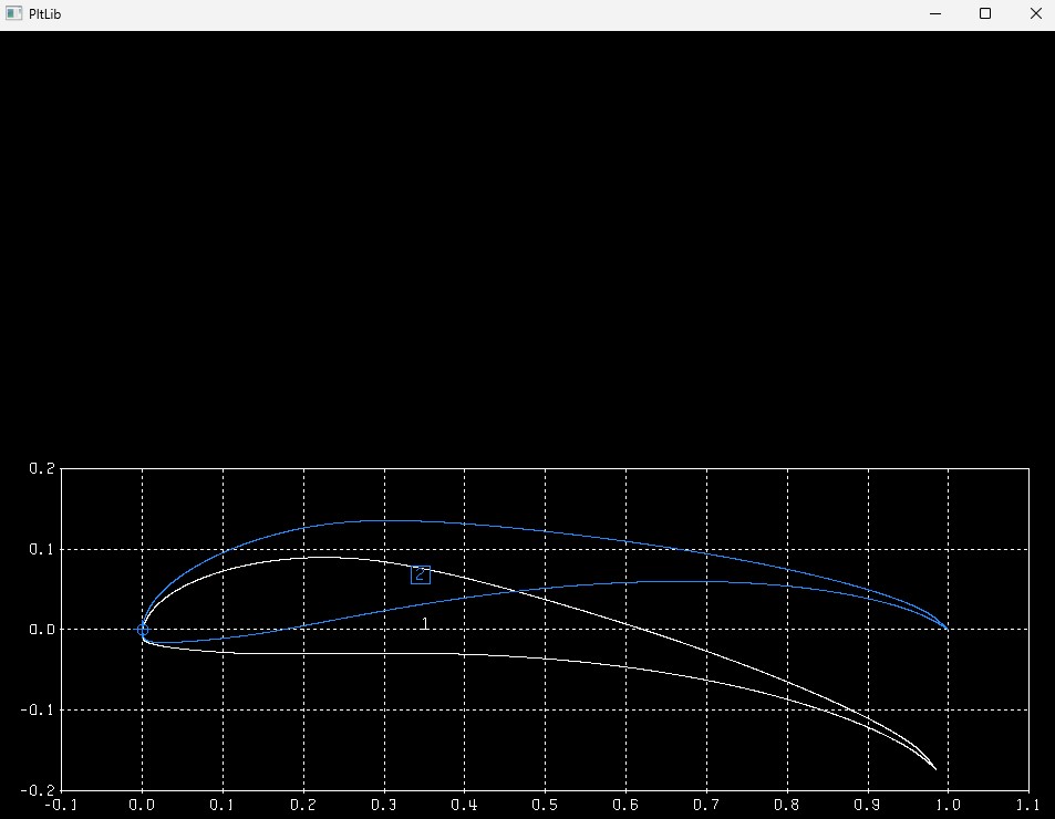
Fig. 10 2 elements in the GUI
Now, type “M” to move it to your desired coordinate. Type in your X and Y coordinates as shown below, and hit enter.
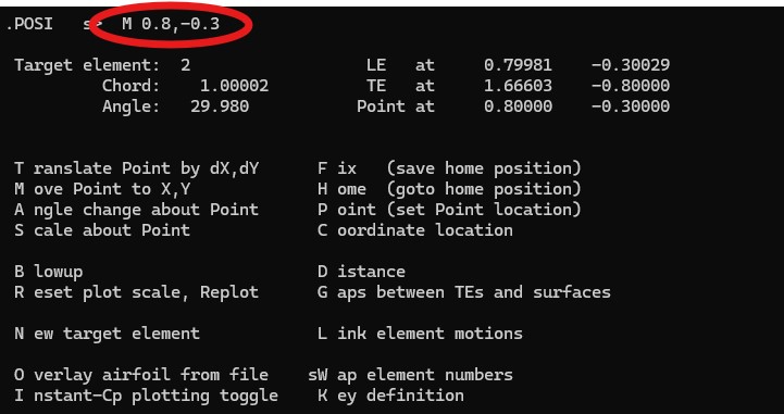
Fig. 11 "M" command
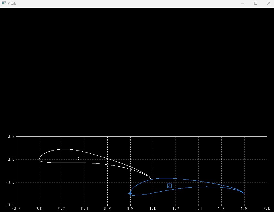
Fig. 12 Secondary element moved to desired coordinates
I’m going to change the AoA of the second element to +30deg using “A.”
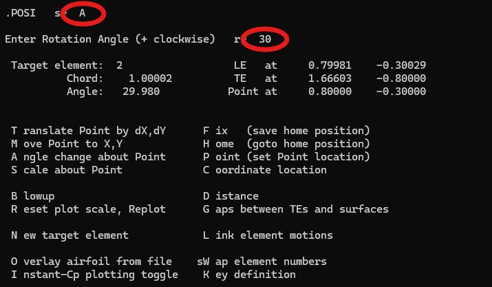
Fig. 13 AoA to 30deg
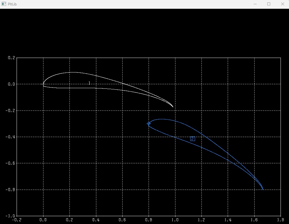
Fig. 14 AoA updated in GUI
If you want to scale it down, type “S” and type in your scaling about the element’s point. I highly recommend uniform scaling so you don’t morph the established profile into some other shape you don’t want.
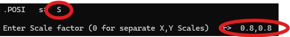
Fig. 15 Scaling second element down to desired size
Once you are happy with your second element, you can hit enter again and type in the filename of another profile to continue adding airfoils to your setup.
Once you are done setting up your airfoils, hit enter twice to get back to the airset menu. Note, that in any menu, you can type “?” to view a list of commands.
Once back in airset, type “Save” to save your airfoil setup. Enter “blade” as the filename. If it is anything other than blade it will not work, and at the current point in time I’m not sure why.
Just type “blade” and hit enter.
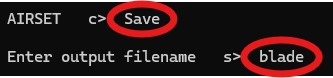
Fig. 16 Always make the filename "blade"
You can now close the airset terminal.
Section summary
- Download the “Selig format dat file” for your profile(s) from airfoiltools.com
- Use airset and it’s list of commands to add and modify your airfoil geometry as you see fit
- When saving your airfoil setup, name it “blade”
mset
Open mset.
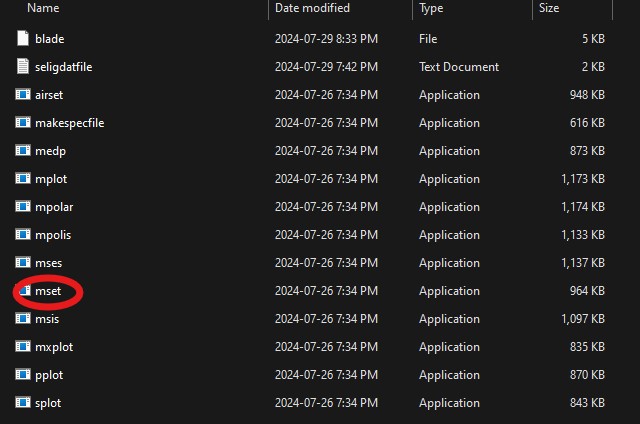
Fig. 17 Open mset
You will be greeted with a menu of 16 commands. Each command is issued with the associated number.
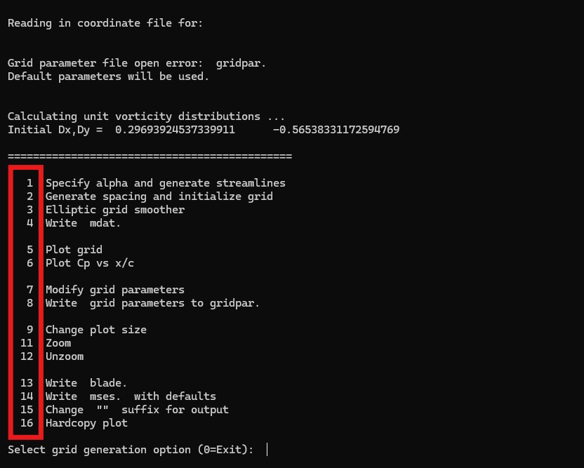
Fig. 18 mset commands
Command 1 is used to specify an AoA of the entire setup. Considering the AoA of each element was already setup using airset, it’s quite rare you want to change the full setup AoA (but there is a chance you might want to, for some reason).
For now, I’m going to use the AoAs specified in airset.
Type “1” and hit enter. Enter your desired setup AoA, and hit enter. A GUI should pop up which looks like the one below.
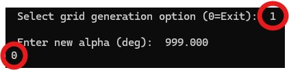
Fig. 19 Entering full setup AoA
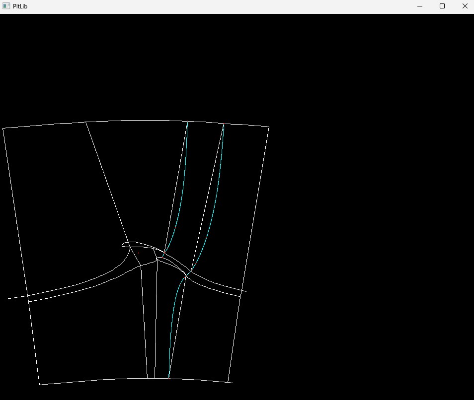
Fig. 20 Streamlines
Type “2” to generate the grid (aka mesh). It will ask you if you are okay with the current mesh shown in the GUI. The generated meshes are usually very good, however if you run into problems/unrealistic values in your solution later on, it would be a good idea to re-visit this step.
Hit enter for each element after you have checked the grid.
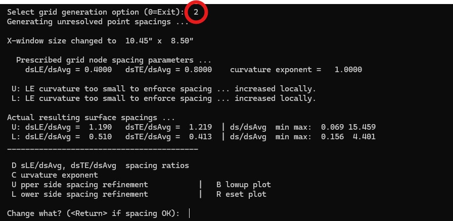
Fig. 21 Grid generation
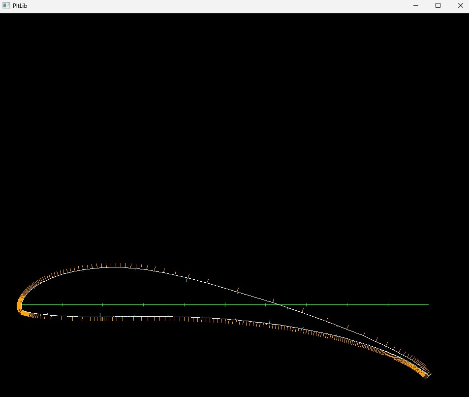
Fig. 22 GUI showing the generated grid. The generated grid is usually good enough for a very accurate solution
Type “3” and hit enter to smooth the grid.
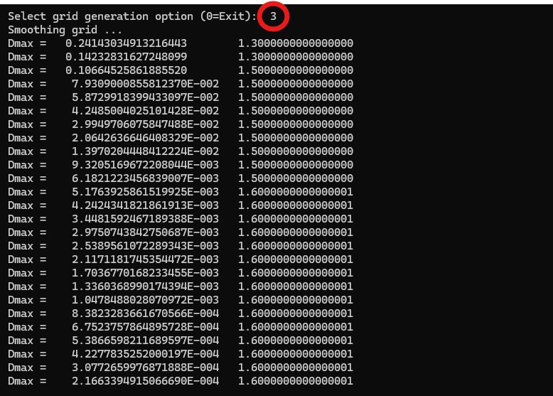
Fig. 23 Smoothing the grid to be easily computed during the solution
Type “4” and hit enter to generate the “mdat” file. This is the file which stores your final solution.
Type “14” and hit enter to generate the “mses” file. This file contains boundary conditions for your simulation. The ones which concern us are the Mach number and Reynolds number.
Find “mses” in your project folder (the file, not the program) and open it with notepad.
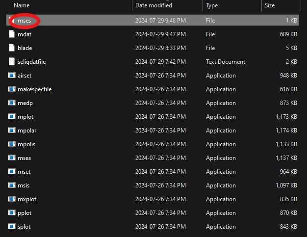
Fig. 24 Generated mses file
You should see the following in notepad. We are mainly concerned with changing our “MACHin” and “REYNin” variables to what we want.
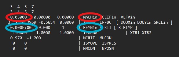
Fig. 25 MACHin and REYNin
You might be wondering why it takes in the Mach number to begin with. When it comes to aircraft, the air flowing over the low pressure side of an airfoil could well exceed Mach 1, despite the incoming freestream air being below Mach 1. High Mach numbers introduce compressibility effects, shock waves, and drastic changes in the fluid properties. Reynold’s number alone won’t capture these phenomenon, which is why the “mses” file asks for it.
For FSAE, the Mach number is entirely irrelevant to the numerical solution, however we are still going to calculate it and input it into our “mses” file for our own knowledge.
From Justification for Aerodynamics we already determined the average FSAE cornering speed is 13.33mps. I’m going to use 15mps since it is a nicer number. Inputting this into a Mach number calculator with SATP taken into account for air temperature, we get Mach=0.04334. Input this value into “mses.”
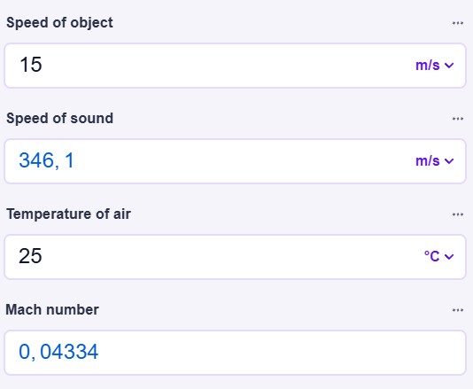
Fig. 26 Mach number calculation
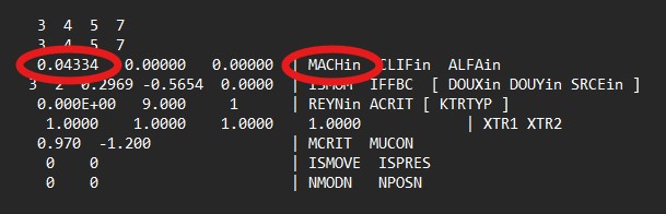
Fig. 27 Inputting Mach number into "mses" file
When calculating Reynolds number, use the chord length of the scaled up airfoil setup as your reference length. In order to do this, we will need to create a copy of “blade” and modify it so that we can import it into SOLIDWORKS.
Make a copy of “blade” and name it “solidworks.”
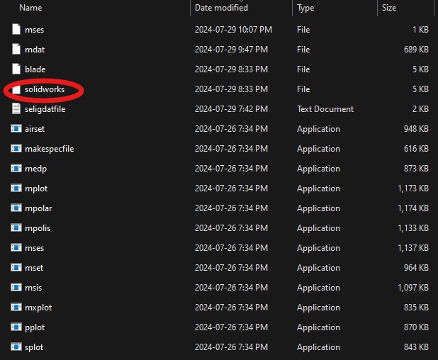
Fig. 28 Coordinate file we will use for SOLIDWORKS
Copy and paste everything from “solidworks” into TXTformat.
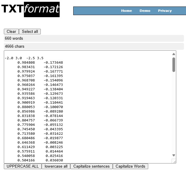
Fig. 29 Using TXTformat to get coordinate file ready for importing into SOLIDWORKS
Delete the first 2 rows, and use the “Trim” tool to trim the first 6 characters of each line.

Fig. 30 Your TXTformat should look like this
Scroll through and find the line which contains “999.0” and delete it.
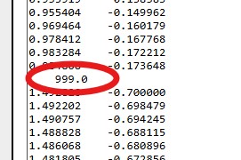
Fig. 31 Before deleting 999.0
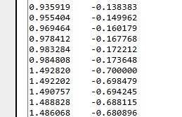
Fig. 32 After deleting 999.0
Use the “Replace” tool to replace “ “ (5 spaces) with “, “ (1 comma, 1 space). Use “Replace” again to replace “ -“ (4 spaces, 1 negative sign) with “, -“ (1 comma, 1 space, 1 negative sign).
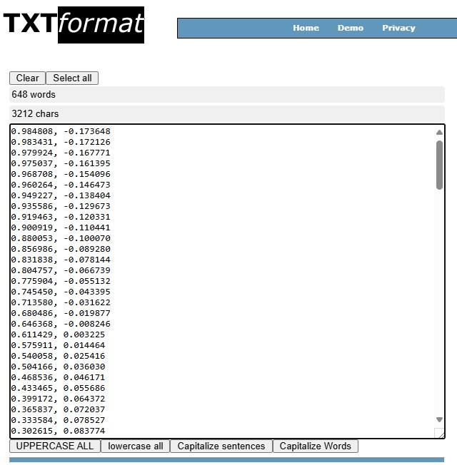
Fig. 33 Your TXTformat should look like this
Use the “Add” tool to add “, 0” (1 comma, 1 space, one 0) to the end of each line.

Fig. 34 Your TXTformat should look like this
Make a new notepad file, name it “solidworks1” and copy and paste your formatted text into it. Save “solidworks1” to your project folder. Be sure to save it as a .txt file.

Fig. 35 solidworks1 contents
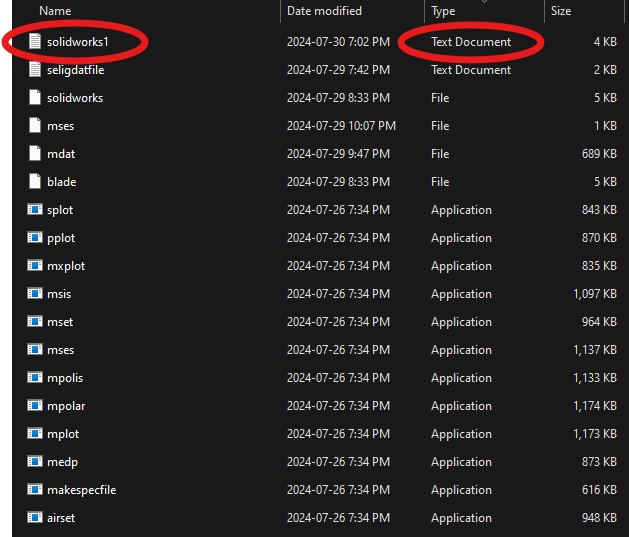
Fig. 36 solidworks1 directory
Within “solidworks1” find the coordinate which differentiates your elements. This can be easily identified by a large change in the x-coordinate. Make an empty line there.
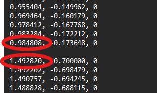
Fig. 37 Large jumps in x-coordinate indicate a new element. Add an empty line between the 2 coordinates
Make a new .txt file in notepad called “element1” and copy and paste the coordinates of the first element. Save the file to your project directory. Repeat this step for every element you have.
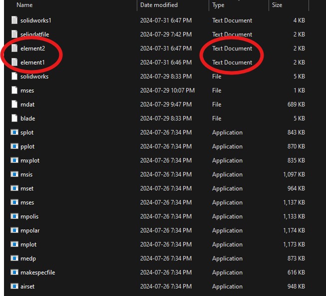
Fig. 38 Coordinate files for elements 1 and 2. Repeat for as many elements as you have in your setup
Open SOLIDWORKS and make a new part file called “wing.” Navigate to Insert –> Curve –> Curve Through XYZ Points.
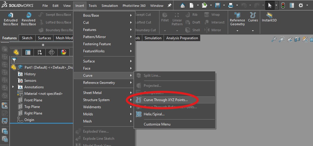
Fig. 39 Tool used to insert airfoil coordinates
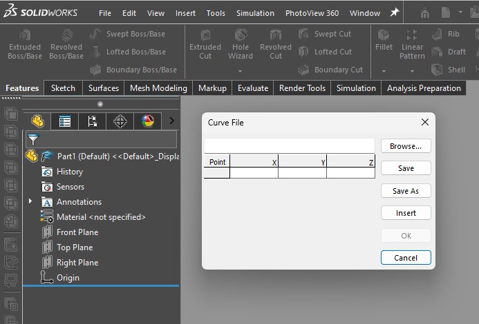
Fig. 40 XYZ Curves menu
Click “Browse…” and find your first element file. Make sure to set the search restriction to text files in your file explorer window.
Open “element1” then click “OK.”
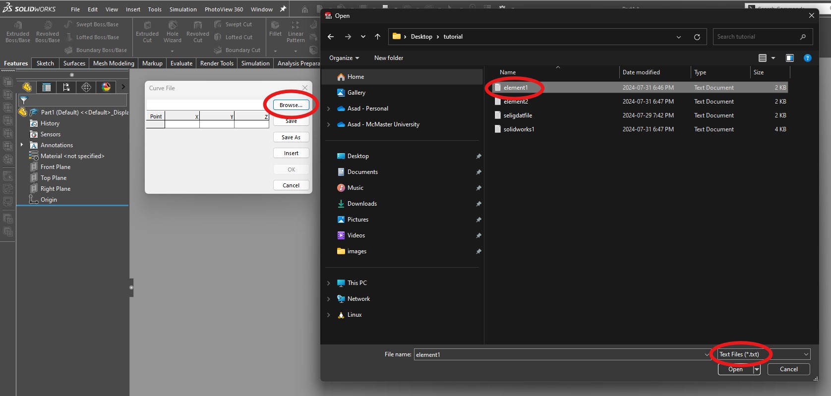
Fig. 41 Inserting first element
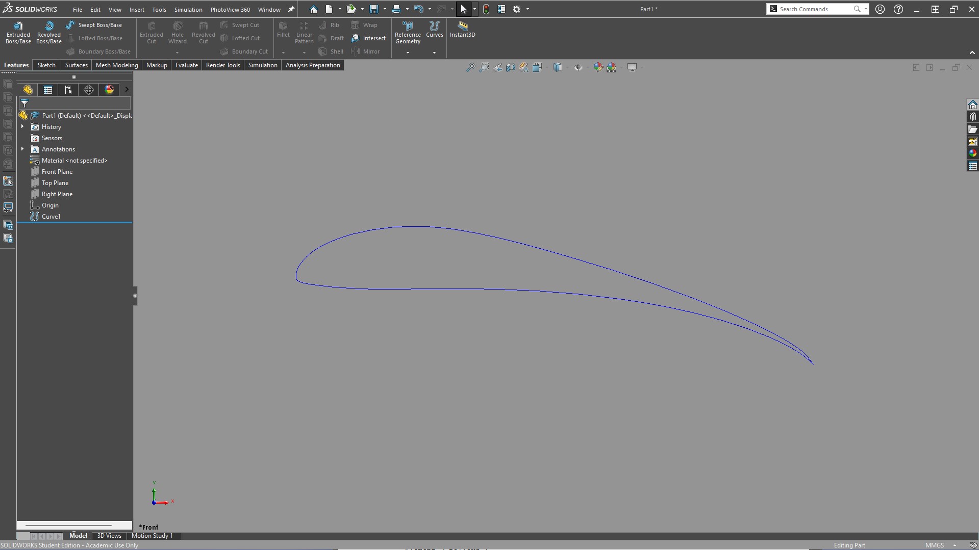
Fig. 42 Inserted first element into SOLIDWORKS
Repeat for all remaining elements.
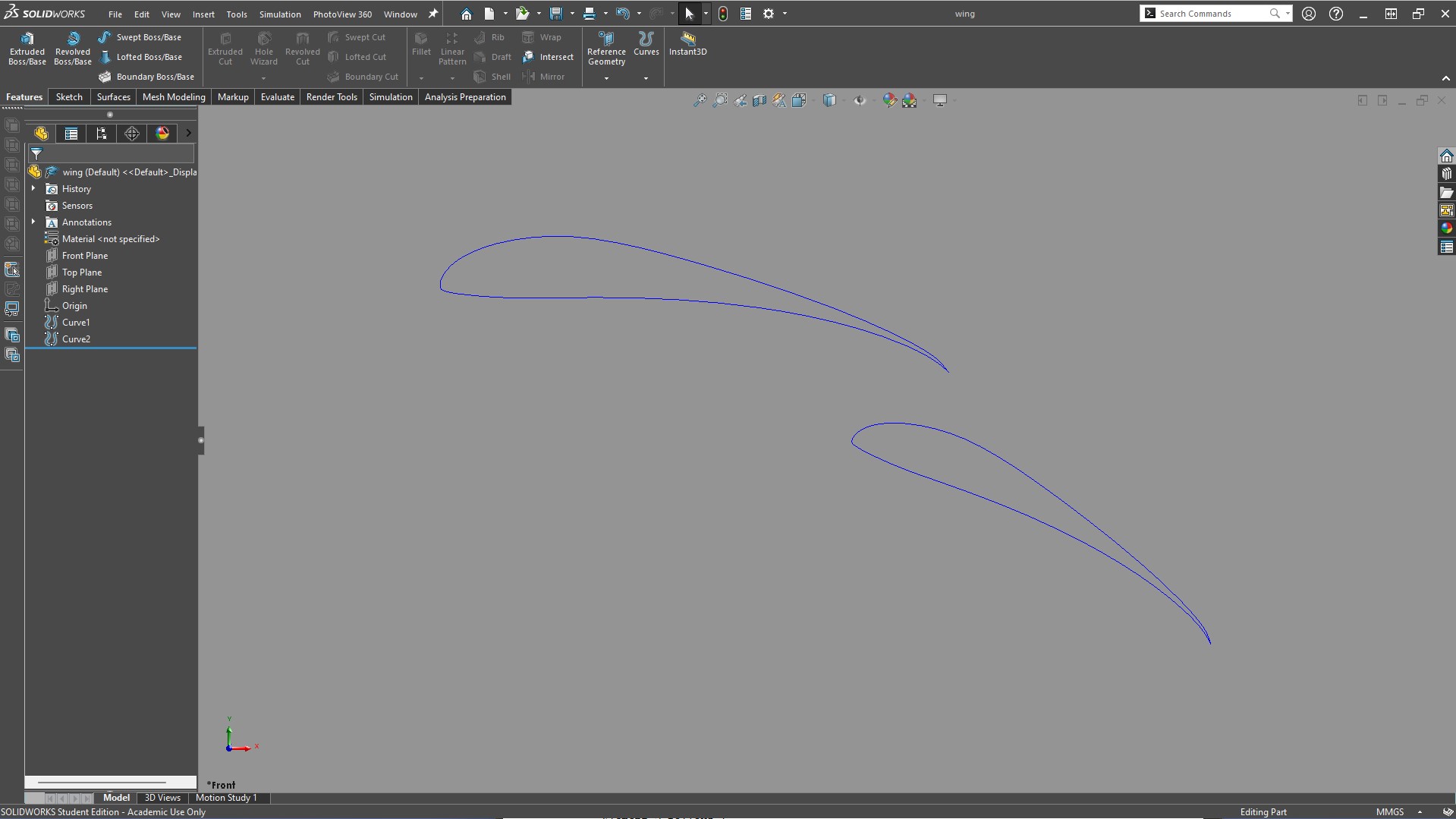
Fig. 43 Full wing setup in SOLIDWORKS
Make a new sketch on the front plane and draw a horizontal centerline at the origin. Convert the curves to sketches, and mirror them about the centerline. Make sure to uncheck “copy” before you mirror the sketches, otherwise you will get errors.
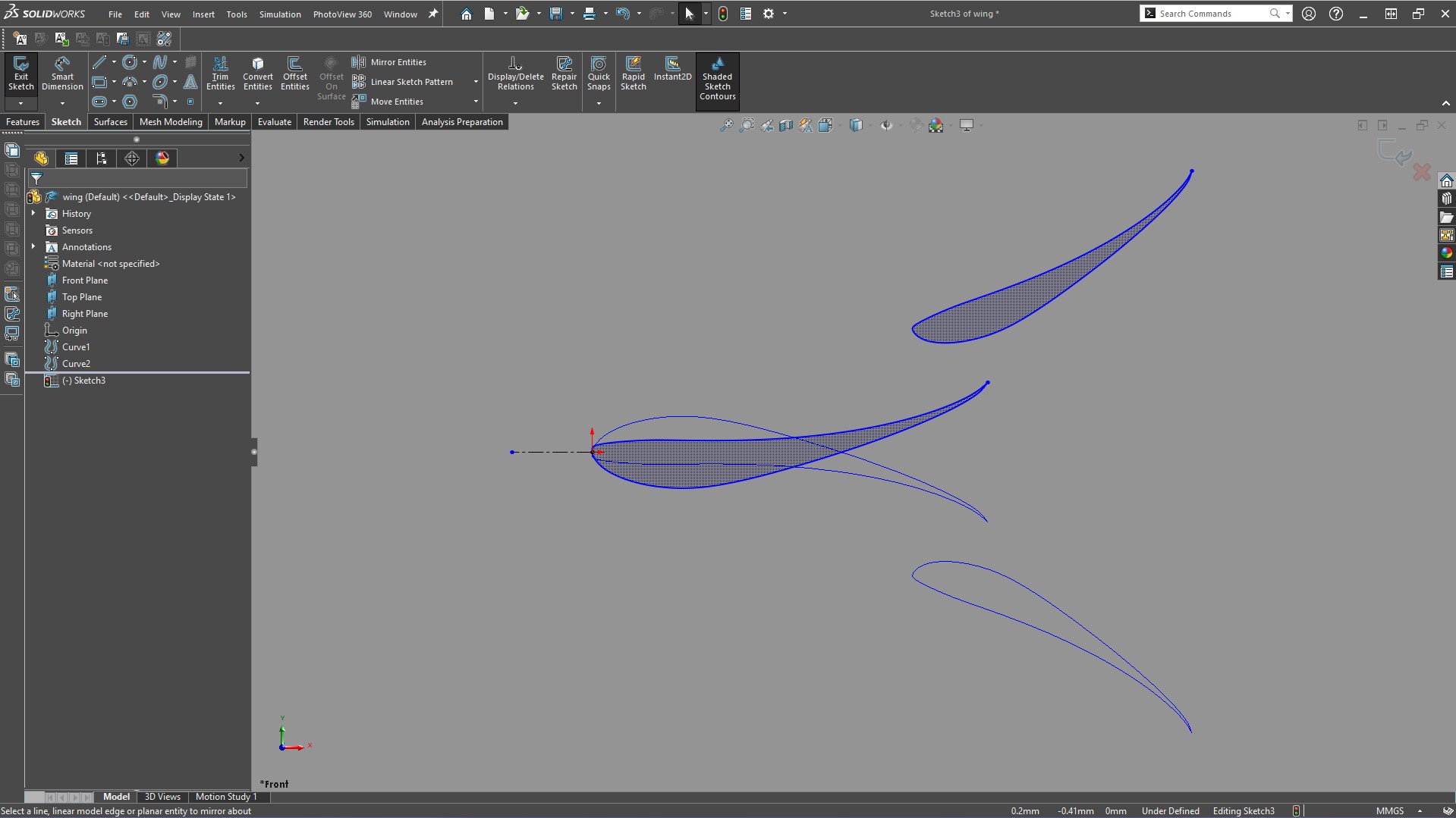
Fig. 44 Mirrored wing setup
Hide the curves, and delete the centerline. Navigate to Tools –> Blocks –> Make and turn the entire sketch into a block.
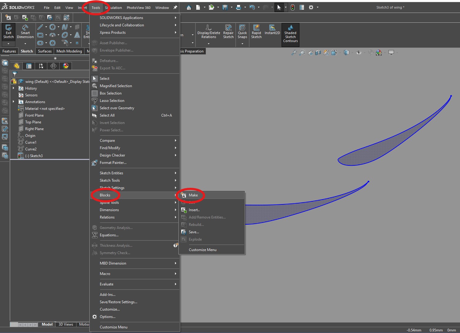
Fig. 45 Make a block
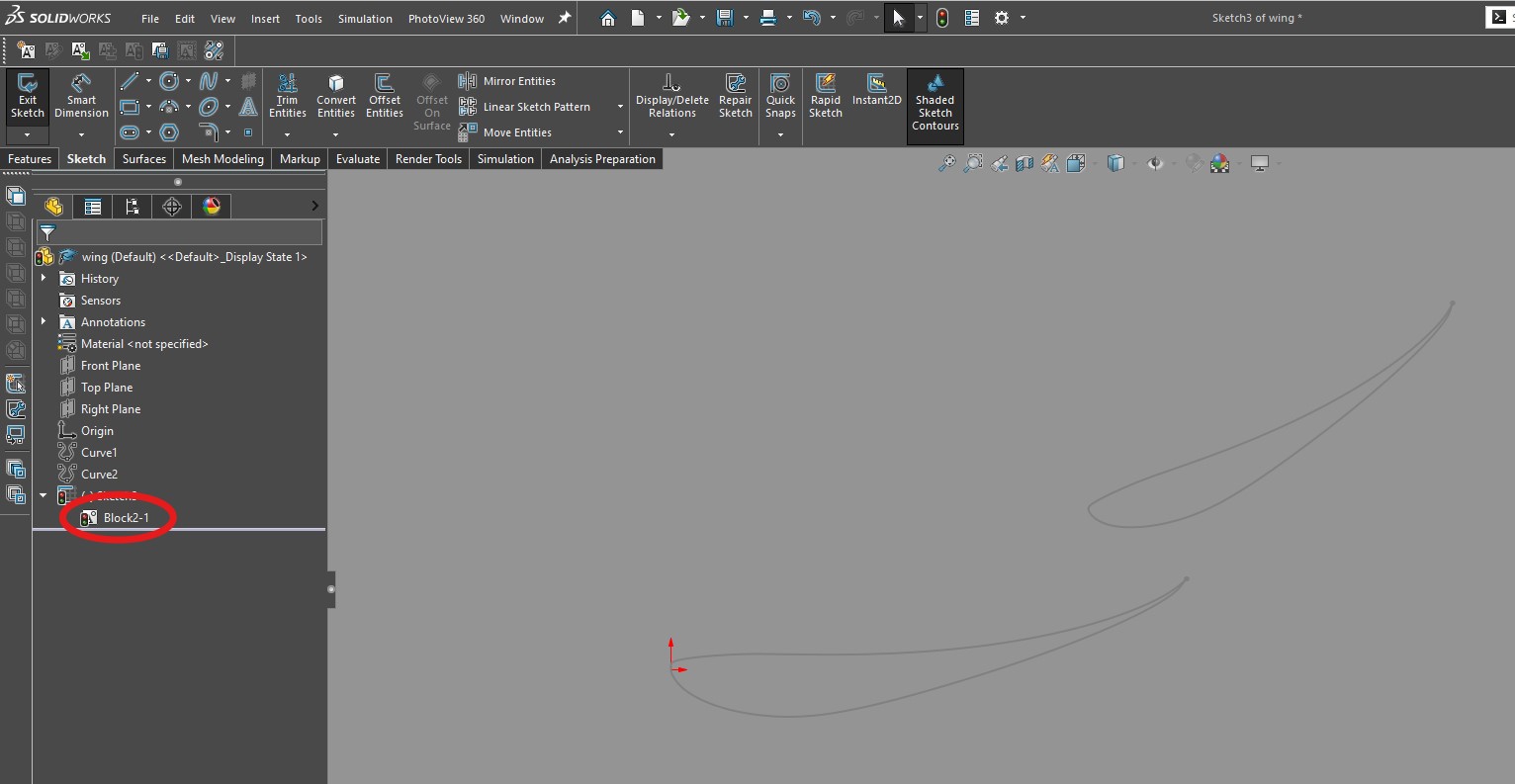
Fig. 46 Block
Left click on the block in the SOLIDWORKS GUI, and you should see a menu pop up on the left. Change “Block Scale” to the desired scale.
For example, if I wanted the primary element’s chord length to be 500mm, I will enter a scale factor of 500.
Exit the sketch.
Make a new sketch on the front plane, and convert the block to a sketch as shown below.
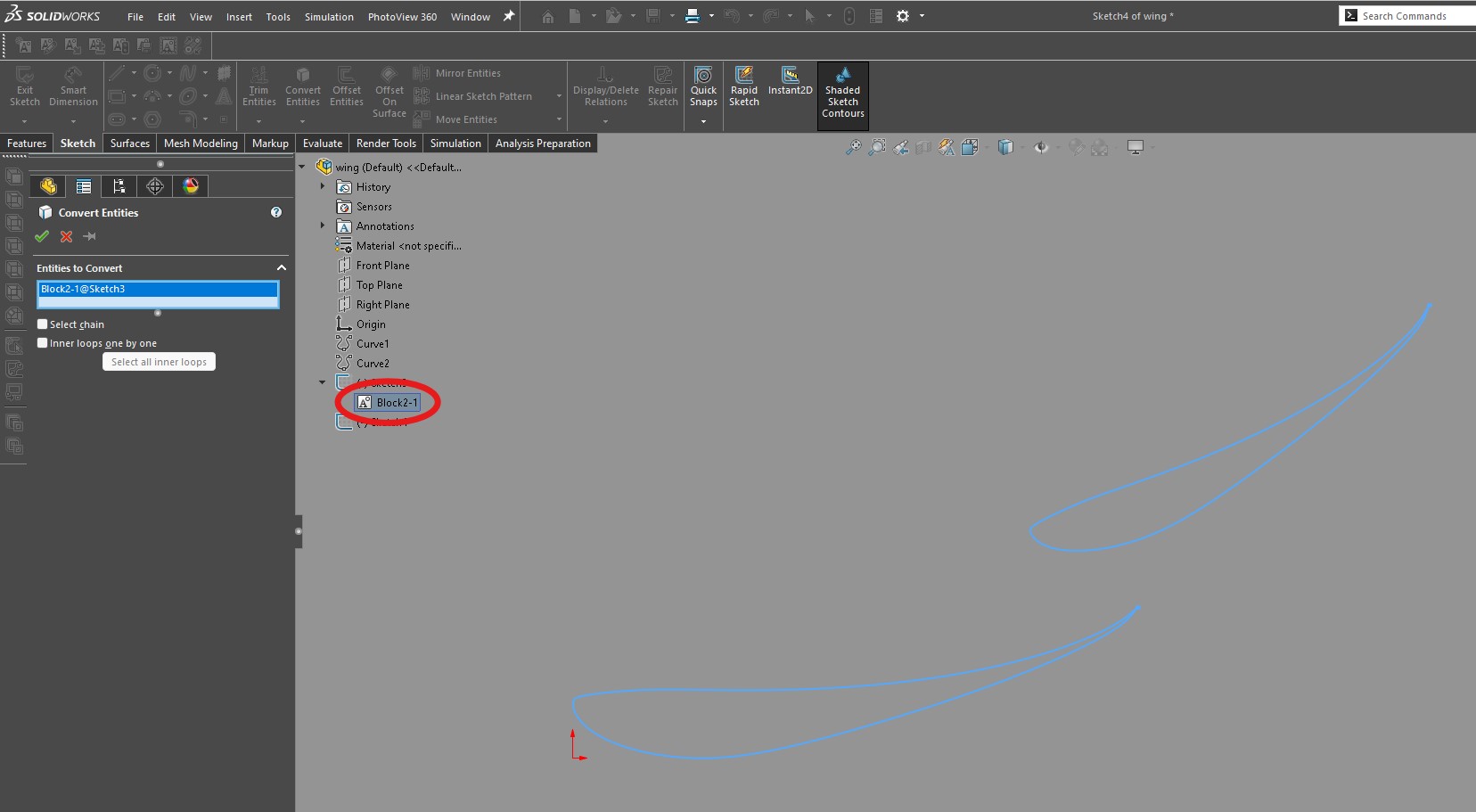
Fig. 47 Converting block to a sketch
Hide the old sketch (the one which contains the block in it). Define the chord length of element 1 (which MACFE aerodynamics people should already know how to do!) and draw a line from the first element’s leading edge to the last element’s trailing edge. Measure the distance of this line. This is the global chord length of the wing.
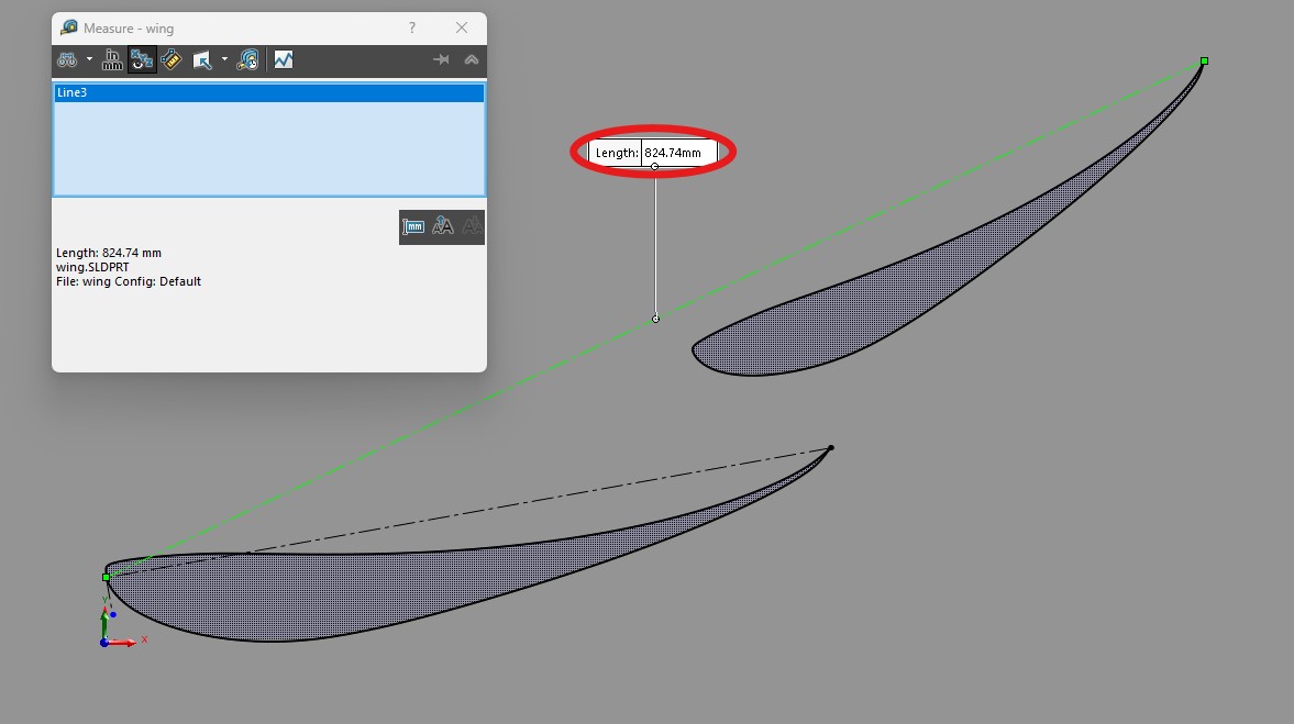
Fig. 48 Global chord length of wing
Save the part file, and close it.
We are now going to use this global chord length to calculate the Reynolds number of our wing.
Go to Reynolds number calculator and calculate Reynolds number under SATP. Below is the Reynolds number of the wing setup I am using for this tutorial.
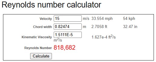
Fig. 49 Reynolds number of wing setup
Input this into the “mses” file.
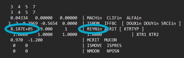
Fig. 50 REYNin
Save and close the “mses” file.
Section summary
- Use “mset” to generate your mesh, and your “mdat” and “mses” files
- Calculate “MACHin” using inlet velocity
- Calculate “REYNin” using inlet velocity and global chord length, which you get from the scaled up wing in SOLIDWORKS
makespecfile
Open “makespecfile.”
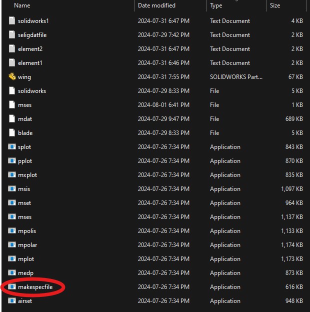
Fig. 51 makespecfile
Hit enter when prompted to enter an extension. Type “5” and hit enter. Enter the full setup AoA twice (for this tutorial, the full setup AoA is 0deg). Enter “0.1” for the “delta parameter value.” The program should automatically close.

Fig. 52 Values to enter into makespecfile
mses
Open “mses.”
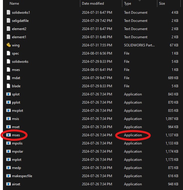
Fig. 53 Open mses (the application, not the file!)
When prompted to enter the number of iterations, enter 50. The program should run for 50 iterations. Close the program after it is done running.
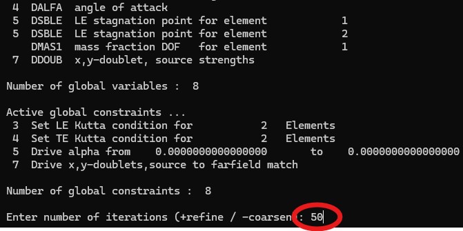
Fig. 54 Run mses for 50 iterations
mpolar
Open “mpolar.” The program should run then close.
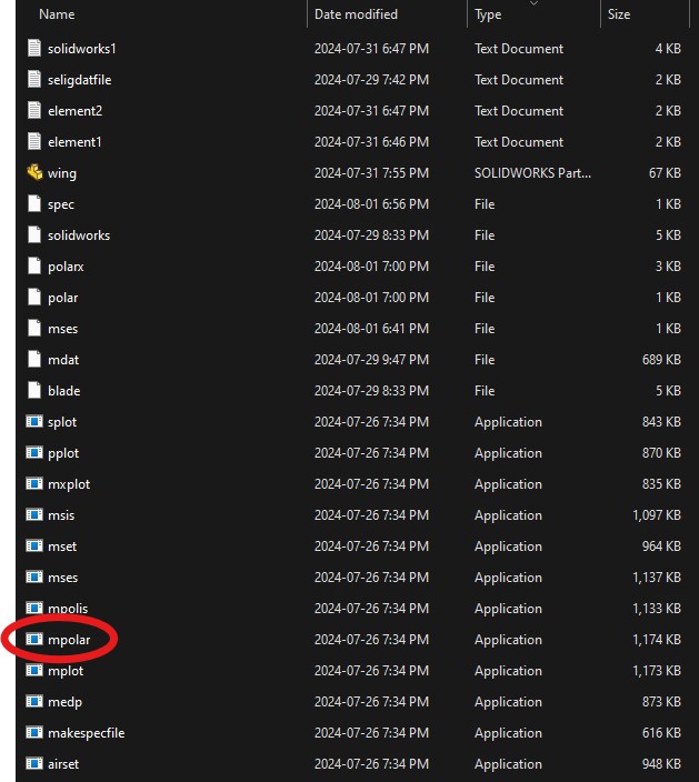
Fig. 55 mpolar
mplot
Open “mplot.”