Unstructured Multi-Element 2D Workflow
MSES did not want to plot results for cases with large amounts of flow separation. For FSAE we need to be able to push into the flow separation regime to find the optimal multi-element wing setups.
Below is the new 2D CFD workflow MACFE will follow, and it uses unstructured meshes. Included in this article is the error between structured and unstructured meshes and Selig’s experimental data.
This one is less of a tutorial, more of a guide. Hope it helps.
Geometry
Not using fluent meshing for this workflow since fluent currently does not support disconnected 2D surfaces (which is what this is).
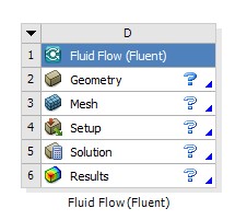
Fig. 1 Non-fluent meshing
Import geometry as .STEP file, change analysis type to 2D, and open in Spaceclaim. Fluid domain should be 6 chord lengths from the wing in all directions except the outlet. The outlet should be 12 chord lengths away from the airfoil. This is based on personal experimentation working well when comparing with wind tunnel data.
Nearfield should be 2 chord lengths from wing. Extends to outlet. Farfield should be 4 chord lengths from wing. Extends to outlet.
Note: make sure to use the global chord length for multi-element setups. For this walkthrough I’m using single element since I need to compare it to wind tunnel data at the end.
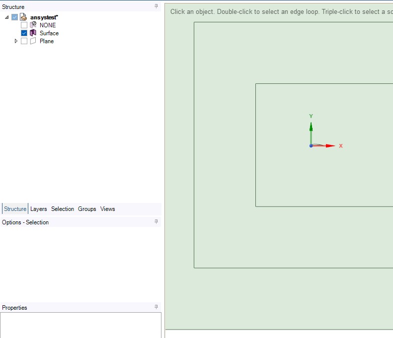
Fig. 2 Domain sizing. Be sure to suppress the wing CAD for physics, since it is captured in the domain
Create your named selections accordingly.
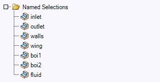
Fig. 3 Named selections
Mesh
Insert “All Triangles Method.” This is the basis of our unstructured mesh. Triangles have been proven to work better around curved geometry in rectangular domains, compared to traditional square cells. Skewed squares near the trailing edge really threw off results in my experiments. Triangles handle it better.
Calculate your y+ value. Use dynamic viscosity of air at SATP, which is around 0.00001849 kg/m-s.
My freestream velocity is 9.07m/s since it corresponds to Re=300,000 for my chord length. This will allow me to compare it to Selig’s data at the same Re.
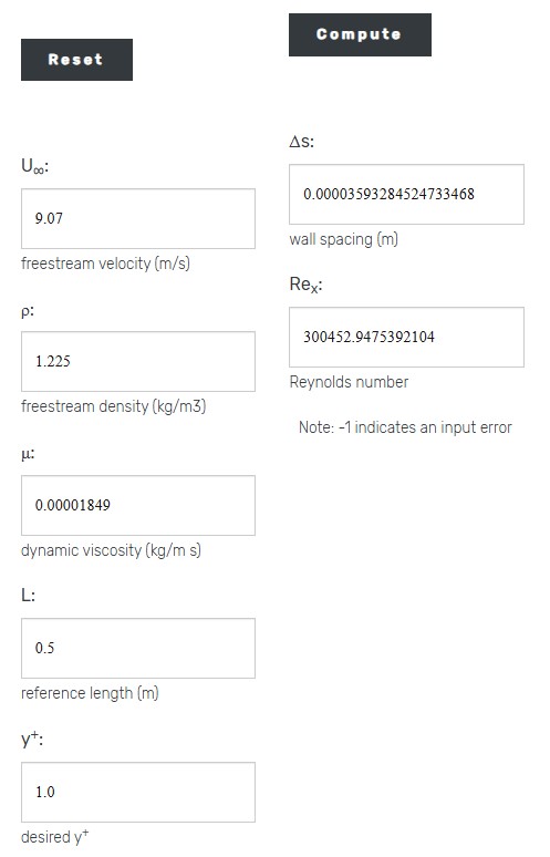
Fig. 4 Computed y+ of 0.03mm
Insert the “Inflation” task and enter your y+.
Note: 25 inflation layers is great for accuracy, however you may need to reduce it to prevent meshing errors in multi-element setups.
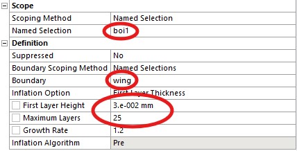
Fig. 5 Inflation layers for wing
Insert edge sizing for wing. For a half meter chord, 0.1mm long cells are usually good. In general, try to use as many divisions as possible before your mesh becomes too fine and your solution starts to break down (it will break down when using coupled solvers with non-negligible viscous effects).
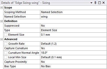
Fig. 6 Edge sizing for wing
Insert face sizings for the nearfield, farfield, and the rest of the mesh. I found 8, 16, and 64mm worked well respectively, however this is just a guide. Do your own mesh sensitivity studies, always.
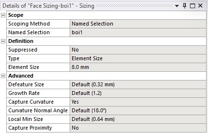
Fig. 7 Nearfield sizing
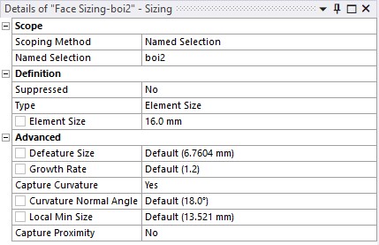
Fig. 8 Farfield sizing
Set your target skewness. I’m going for 0.7 which, again, I’ve found to work well for getting accurate data. Try to get the lowest possible skewness without sacrificing compute time.
Just be sure to not get lost in the sauce trying to get a pixel perfect mesh. You still have the rest of the design and analysis process to go through. And don’t forget how long manufacturing takes…
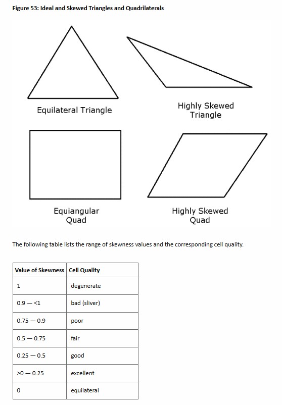
Fig. 9 Definition of skewness from Ansys documentation
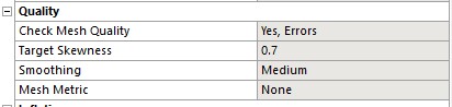
Fig. 10 Setting target skewness under "Mesh --> Quality --> Target Skewness"
Generate your mesh. This will take 3-15 minutes depending on your hardware. If it takes longer than that, get better hardware.
Last step for the mesh, set “Send to Solver” for boi1 and boi2 to “No.” Otherwise you will not be able to run your sim.
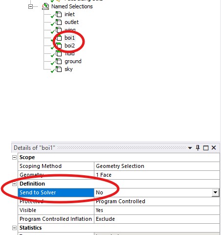
Fig. 11 Disable send to solver for all BoIs
Setup
Be sure to enable double precision for improved accuracy, and enter the total number of cores available on your machine. Enable your GPU(s) under “Parallel Settings” if you have any.
Input your velocity boundary condition. Set your ground and sky to “inviscid” condition (specified shear of 0 Pa). Make sure the wing is set to no slip condition.

Fig. 12 Inviscid ground, do the same for sky
If you are doing a ground effect study, set the ground to translating at the desired velocity, as shown below.
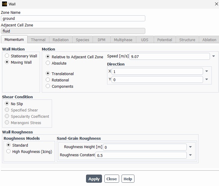
Fig. 13 Ground effect BC
Create your monitors for Cl, Cd, and anything else you want, and make sure you print to console so you can view the results during the solve.
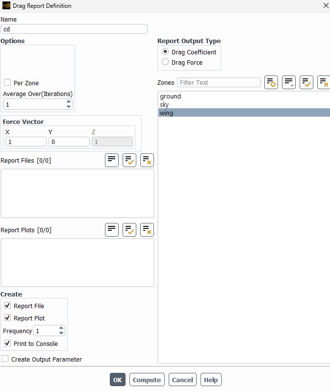
Fig. 14 Report monitors
Set your reference values. For 2D CFD, your reference area is chord*depth, meaning if your depth=1m your chord is simply your reference area, which simplifies things a lot. So, for practical purposes, keep your depth=1m always.
Enter your length (chord, global chord for multi-element) and velocity as well.
Just for the reader’s knowledge, these reference values are only used when calcualting Cl and Cd to output to the console. However the values entered in the BCs are what ultimately matter since that is what Ansys uses when solving.
So for your own simplicity, make sure your reference values and BCs are the same.
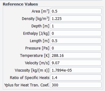
Fig. 15 Reference values
Set your turbulence model. I highly recommend reading the Ansys documentation for k-w SST w/ Intermittency to understand why these models are used, and to get an intuitive feeling of how they affect the solution. Below are some useful links which are good to read up on.
| k-w SST turbulence model | https://ansyshelp.ansys.com/account/secured?returnurl=/Views/Secured/corp/v242/en/flu_th/flu_th_sec_turb_kw_sst.html |
| Intermittency transition model | https://ansyshelp.ansys.com/account/secured?returnurl=/Views/Secured/corp/v242/en/flu_th/flu_th_sec_turb_intermittency_over.html?q=transition%20model |
| Near wall treatment for w-based turbulence models | https://ansyshelp.ansys.com/account/secured?returnurl=/Views/Secured/corp/v242/en/flu_th/section_kbf_dl4_vvb.html?q=k%20omega%20sst%20near%20wall |
Again, for the reader’s own knowledge, enhanced wall functions are automatically applied to the k-w SST turbulence model in Fluent. Wall functions are applied when y+ is greater than 30 (in the logarithmic layer).
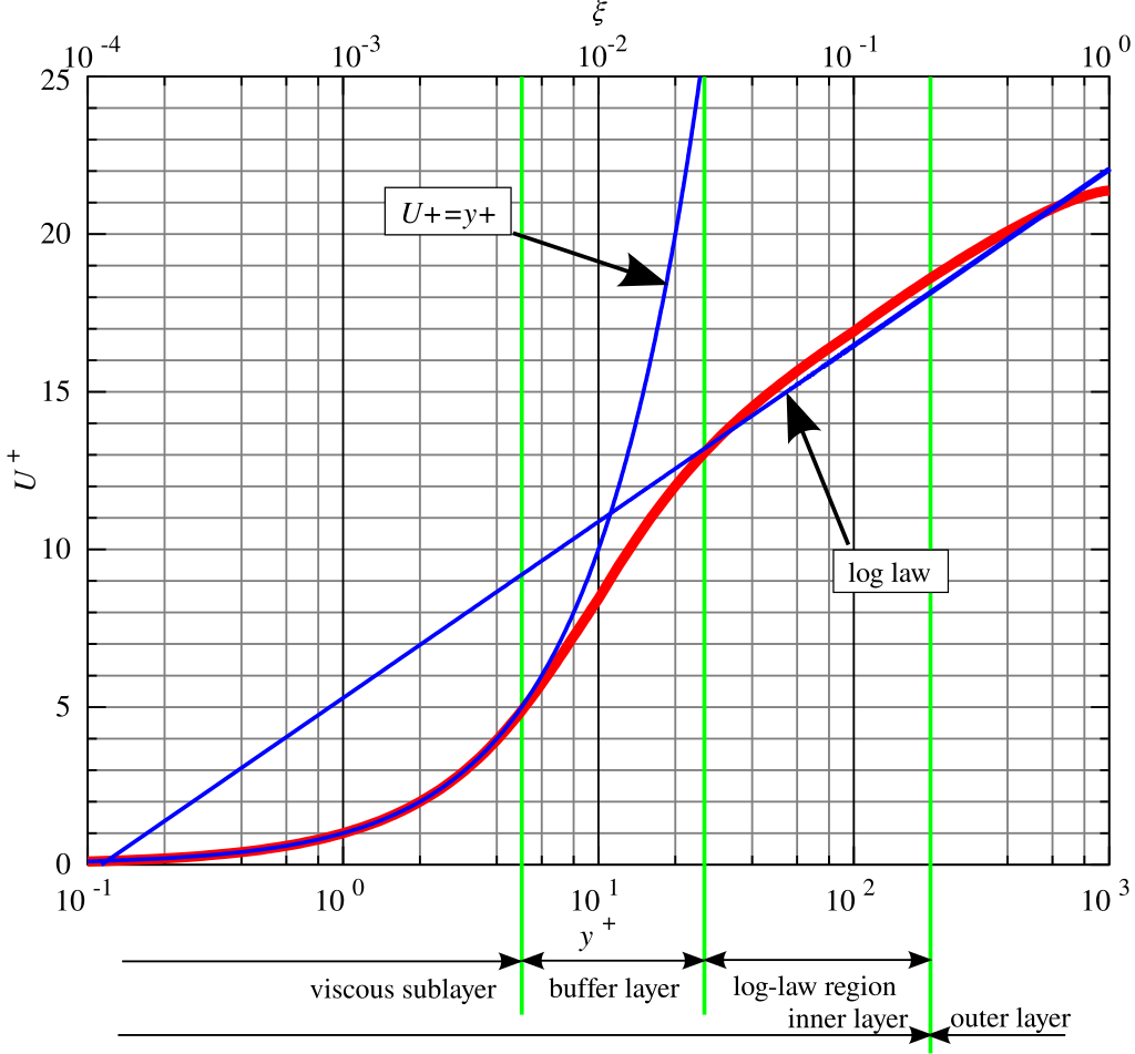
Fig. 16 Law of the wall
The y+ insensitive near-wall treatment for w-based models transitions between the lowRe formulation (y+ less than 5) to the highRe formulation (y+ greater than 30) in the best way possible.
Anyways, back to 2D CFD. Below should be your turbulence/transition model settings.
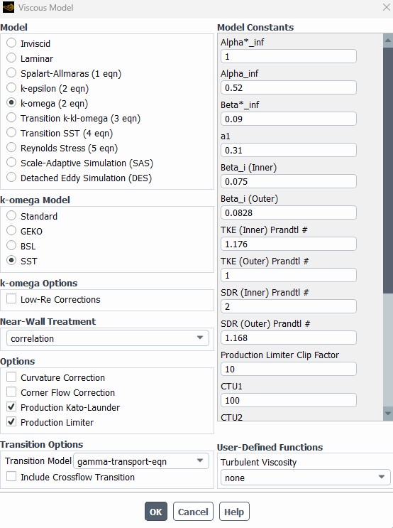
Fig. 17 k-w SST w/ Intermittency
Add convergence conditions for Cl and Cd so you continue to run your simulation beyond Ansys’ default convergence criteria.
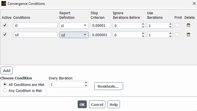
Fig. 18 Convergence conditions for Cl and Cd
Run your solution for 1000 iterations minimum. 3000 iterations is ideal if you have time.